Download PDF
Download page SBG EKF modes of Operation.
SBG EKF modes of Operation
sbgEkf Introduction
Thanks to a modern processing architecture, SBG Systems inertial systems run a real time Extended Kalman Filter (EKF). The coupling between GPS/GNSS and inertial sensors allows GNSS data correct any inertial drift, while keeping high frequency navigation outputs, with excellent performance.
More than just a direct EKF implementation, the implemented algorithms include advanced error models and wrong measurement detection to ensure that best navigation performance is provided at any time.
A modular design allows a wide range of aiding sensors to be connected to the INS. GNSS, Odometer, DVL and other aiding sensors can be connected to further enhance navigation performance.
In addition, the Extended Kalman filter is able to estimate some user entered parameters to further improve accuracy, such as GPS lever arm, odometer's gain, and others.
Specialized motion profiles and error models provide optimal options and tuning for each application, and each aiding equipment.
Basic principle
Inertial sensors (accelerometers and gyroscopes) provide very accurate short term motion measurements but suffer from drift when integration time becomes long. Some other systems such as GNSS receivers or odometer provide low frequency measurements that can be fooled by jamming, or short term measurements errors, but these sensors provide good performance over long term.
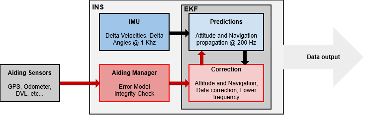
The basic idea behind the Kalman filter is to take the best of each sensor, without drawbacks. A high frequency prediction (also called propagation) step uses inertial sensors to precisely measure motion and navigation data. When aiding data (GPS position, Odometer data or DVL reading for example) becomes available, the Kalman filter will use it to correct the current state and prevent drift.
As aiding measurements are made at a lower frequency than the prediction step, a small jump can be observed after a correction is applied. This jump should be really small in normal operating conditions.
A covariance matrix maintains up to date each estimated parameter error. When there is no measurement available, estimation error tends to increase; when a new measurement is received, this error will decrease. This covariance matrix is also used to handle the “link” between each estimated parameters.
Besides the EKF, a sensor manager is implemented to check aiding measurements and reject bad ones.
To summarize the EKF operation, the following diagram shows how IMU and external sensors are used
Mode of Operation
The Kalman filter will run into several computation modes depending on situations.
Uninitialized mode
This mode is observed at startup only. Prior to the first attitude computation, the filter is identifying the average direction of gravity using accelerometer. This mode assumes low accelerations so best initialization is achieved when the device is powered up stationary or at constant speed. If the INS is powered up during motion, the full accuracy may be reached within a few minutes after startup.
Vertical Gyro mode
Once roll and pitch angles are initialized, the EKF filter is running in a vertical gyro mode, where only roll and pitch angles are estimated. This mode uses a vertical reference and internal gyroscopes to estimate orientation. Therefore, heading angle is freely drifting. Ship motion data is provided but may have degraded accuracy in dynamic environments.
In this mode the performance is dependent on the dynamics of the vehicle. Performance can be affected during high acceleration maneuvers.
Heading Rough alignment procedures
This section only applies in case the unit is configured to operate in AHRS or INS modes of operation.
While being operated in “vertical gyro” mode, the EKF is continuously trying to make a first heading angle alignment using different procedures. These procedures have some constraints and the following table explains how they are used and in which situations:
| Method | Availability | Constraints - Remarks |
|---|---|---|
| Magnetic Heading | When Magnetic heading aiding is enabled. | This mode is common for entry level applications, with no high precision requirement. If magnetometers are enabled, this signal is available at startup. A good magnetic field must be available for proper operation. Other methods are recommended for high precision applications. |
| GNSS Dual antenna Heading | When GNSS dual antenna Heading is activated as an aiding input. | In case the setup allows two GNSS antennas to be installed, this method will be the most convenient. It uses GNSS true heading provided by a dual antenna GNSS receiver to align heading. Good GNSS condition are preferred for initialization in order to avoid multi-path errors at startup. A minimum accuracy of 1° for the GNSS true heading has to be reached, to be used in the solution. |
| Kinematic alignment | In Automotive and Airplane and motion profiles. | This method allows heading alignment for applications where heading is mostly aligned with travel direction (course over ground). It uses GNSS velocity, considering that preferred direction of travel is forward. The device must drive/fly in forward direction, at least at 3.0 m/s. |
| Free Kinematic Alignment | In Helicopter, UAV, marine and pedestrian motion profiles | This method uses relative velocity to define a heading. This allow any motion, in any direction unlike the traditional kinematic alignment methods. In order to operate properly, the device should experience linear acceleration or accelerated turns during a time frame of 5 to 10 seconds. The alignment precision will be driven by the amount of dynamics experienced. |
AHRS mode
Once the heading rough alignment has been performed, the full orientation can be estimated by the EKF. The vertical reference is still stabilizing the roll and pitch angles. Heading is also stabilized thanks to the dual antenna or magnetic aiding. Position and velocity are freely drifting and cannot be considered as valid in this mode.
As for the Vertical gyro mode, the performance can be affected by high dynamic maneuvers.
Position and velocity initialization
As for heading alignment, the system continuously tries to initialize the position and velocity using GNSS inputs when operated in AHRS mode.
Full Navigation mode
In this mode, the EKF provides the full navigation outputs: Orientation, absolute position and velocity are estimated.
The Full navigation mode can use all available sensors input to maintain the best solution, even in case of short GNSS outages.
AHRS - Navigation Mode
AHRS units behavior slightly differ from one product line to another: The Ellipse-A cannot accept aiding data so it only runs in the AHRS mode. However, higher performance motion reference units (MRUs) accept an external GNSS input to allow navigation mode to be used internally. This improves orientation output performance. Only orientation outputs remain available in this case.
Heading Observability
This section is important to understand how a GNSS aided INS is able to track an accurate heading.
Using Single Antenna GNSS
In the most simple setup, with only an INS aided by a single GNSS antenna, the heading is not always observed.
In particular, when de device is subject to static conditions or at constant speed, only roll and pitch angles are accurately corrected, and heading can show some drift (reported on the standard deviation outputs). As soon as the device is subject to acceleration, the EKF will also stabilize heading angle.
In case the reported Yaw angle standard deviation becomes high or the error increases, then doing some dynamic maneuver will improve accuracy. This will help in airborne application with UAVs for example where only a single antenna is available.
Using Dual Antenna GNSS
The heading observation is greatly improved in low dynamic conditions when coupling the INS with a dual antenna GNSS system. In such condition, the INS will be able to provide accurate heading in all conditions, and will cope with GNSS heading outages in case of multipath environment. Dual antenna heading also provides a very accurate heading angle, often required by survey applications.
This option is particularly effective in marine applications which have low dynamics and a high precision requirement.
Automotive applications
In automotive applications, it's often possible to assume that there is no lateral velocity. This assumption allows the filter to optimize its performance. Thus heading becomes fully accurate as soon as the vehicle is driving.
Using a dual antenna heading can further improve heading performance in case the vehicle is regularly in static condition.
Using Magnetic Heading
In many applications such as airborne or sometimes in marine environment, the magnetometer can provide an efficient heading aiding input as long as it is calibrated and used away from magnetic interference. The Magnetic Heading is converted to True heading by using the position and date and the World Magnetic Model 2020.
Magnetic heading is a cost effective way to observe heading in low dynamic conditions but can be subject to degradations in difficult magnetic conditions. Its accuracy is limited to 1° approximately.
Improving Navigation Performance
Lateral velocity constraints
When the "Automotive" motion profile is selected, the EKF assumes that lateral velocity is 0. In addition to improve the heading performance, this will greatly reduce the position drift in challenging conditions such as urban canyons.
Regular turns are required to constrain the velocity in all directions.
Odometer Aiding
In addition to the GNSS aiding, all INS models provide an odometer input which can greatly improve performance in challenging environments such as urban canyons for automotive applications. The odometer provides a reliable velocity information even during GNSS outages. This increases significantly the dead reckoning accuracy.
Compared to using only the velocity constraints, the odometer aiding provides useful velocity information that will be very effective in case of dead reckoning in straight lines or slight turns.
Our products support:
● Quadrature output or compatible odometers with forward and reverse directions.
● CAN vehicle velocity messages (fully configurable) for setup with direct interface with vehicle’s ODBII connector
Odometer integration is made really simple as the EKF will finely adjust the odometer's gain and will correct residual errors in the odometer alignment and lever arm.
Doppler Velocity Log Aiding
In many marine or underwater applications, the DVL is a good choice to improve navigation when GPS is not available. DVL has been fully coupled with the EKF to provide full navigation performance in both bottom tracking and water layer conditions. No calibration is required as the EKF will automatically adjust alignments and gain parameters.
The fusion of DVL data with the EKF can provide very accurate and reliable underwater position data in real conditions. A carefully chosen mission pattern such as a lawn mower one can also dramatically limit the position error growth.
In addition to the Kalman filter integration with DVL, the inertial sensor can store and output back the DVL messages (PD0) for water profiling applications.
ZUPT Mode
The EKF is able to automatically use “Zero Velocity Updates” (ZUPT) in some motion profiles. When the sensor stops moving, the Kalman filter detects the zero velocity condition and uses that information to correct the states, and then limit the position drift.